Dynamic guessing for Hamiltonian Monte Carlo with embedded numerical root-finding
A new algorithm and Python package for a class of difficult Bayesian statistical models
Abstract
Thanks to scientific machine learning, it is possible to fit Bayesian statistical models whose parameters satisfy analytically intractable algebraic conditions like steady-state constraints. This is often done by embedding a differentiable numerical root-finder inside a gradient-based sampling algorithm like Hamiltonian Monte Carlo. However, computing and differentiating large numbers of numerical solutions comes at a high computational cost. We show that dynamically varying the starting guess within a Hamiltonian trajectory can improve performance. To choose a good guess we propose two heuristics: guess-previous reuses the previous solution as the guess and guess-implicit extrapolates the previous solution using implicit differentiation. We benchmark these heuristics on a range of representative models. We also present a JAX-based Python package providing easy access to a performant sampler augmented with dynamic guessing.
Introduction
If a modeller knows that some partially-known quantities jointly satisfy algebraic constraints, they may want to embed a root-finding problem inside a Bayesian statistical model. For example, biochemical reaction networks are governed by partially-known kinetic parameters and often known to satisfy steady-state constraints. Often the root-finding problem’s solution must be found using numerical methods.
Statistical inference for this kind of model is possible using gradient-based Markov Chain Monte Carlo algorithms like Hamiltonian Monte Carlo and its variants, as the parameter gradients of root-finding problems can usually be found. Unfortunately, solving and differentiating root-finding problems in the course of gradient-based MCMC imposes a substantial computational overhead.
In this paper we propose to address this problem by dynamically updating the root-finding algorithm’s starting guess as the sampler moves along a simulated Hamiltonian trajectory. We propose heuristics for updating the guess and test these on a range of models, showing that dynamic guessing improves performance compared with the state of the art. We also present a Python package grapevine containing our implementation of HMC with dynamic guessing, benchmarks and convenience functions that allow users to easily fit their own statistical models using our algorithm.
Our Python package and the code used to perform the experiments reported in this paper are available at [ANONYMISED] and from the Python Package Index.
Related work
Bayesian statistical modelling with embedded numerical root-finding appears in a wide range of scientific contexts, including ignition chemistry
We are not aware of any previous work that developed specialised inference methods for Bayesian models with embedded root finding. Instead, previous work has embedded numerical root-finding within generic inference algorithms such as Hamiltonian Monte Carlo
Hamiltonian Monte Carlo couples the target probability distribution with a dynamical system representing a particle lying on a surface with one dimension per parameter of the target distribution and a potential energy derived from the target density. To generate a sample, a symplectic integrator simulates the particle’s trajectory along the surface after a perturbation. Ideally, the trajectory takes the particle far from its starting point, leading to efficient sampling. The symplectic integrator proceeds by linearising the trajectory in small segments, evaluating the target density and its parameter gradients on log scale at the end of each segment. For targets with embedded numerical root-finding, the roots and their local parameter gradients must also be found at every step.
Many numerical root-finding algorithms are iterative, generating a series of numbers that start with an initial guess and converge towards the true solution. These algorithms tend to perform better, the closer the initial guess is to the true solution: see
Our approach draws on previous work on numerical continuation and warm-starting. Continuation refers to methods that use one numerical solution to generate an initial guess for a perturbed problem, which can then be solved more precisely using another method. For example, an Euler predictor, which perturbs the previous solution using local gradient information, is known to work well with Newton solvers
Methods
Instead of using the same starting guess for every root-finding problem on one simulated Hamiltonian trajectory, we propose choosing the guess dynamically, based on the previous integrator state. We call this approach the “grapevine method” after the expression “I heard it through the grapevine” and the visual resemblance of a simulated Hamiltonian trajectory to a vine, with the numerical solution at each integrator step representing grapes.
We implemented this idea by augmenting the velocity Verlet integrator
For HMC sampling to be valid, it is important that the target probability density function is constant. If all embedded root-finding problems have single roots, this will be the case up to numerical error for the grapevine algorithm, as the guessing heuristic does not affect what solution the root-finder will find, but only how quickly it converges. Therefore in this case there is no difference in MCMC validity between a grapevine sampler and an equivalent sampler with static guessing. If an embedded problem has multiple roots, then the root that the solver finds may depend on the guess, so that the target density is not constant. Users must therefore verify that all embedded root-finding problems have single roots.
We tested two heuristics for generating an initial guess: guess-previous and guess-implicit. The information for the heuristic guess-previous is the solution of the previous root-finding problem. The heuristic is simply to use the previous solution as the next guess. The information for the heuristic guess-implicit is the solution of the previous root-finding problem, and also the parameter values at the previous step. The heuristic is to use implicit differentiation to find the local derivative of the previous solution with respect to the previous parameters, then obtain a guess by perturbing the previous solution by the product of this derivative and the change in parameter values. See Appendix 2 for details of how guess-implicit is defined and implemented.
Experiments
First we prepared an example illustrating the benefit of dynamic guessing by comparing behaviour of dynamic and static heuristics along a single Hamiltonian trajectory. Black crosses show the solutions of 11 root-finding problems (finding the minimum of a parametrised 2-dimensional Rosenbrock function) corresponding to points along a simulated Hamiltonian trajectory through parameter space. Coloured lines show the paths through solution space taken by a Newton solver to approximately solve each problem. Note that some of these paths are very small. Coloured dots indicate the guess used for the current problem. For the first problem in the trajectory all heuristics use the default guess at coordinate (1, 1), whereas the dynamic heuristics subsequently use better guesses that lie much closer to the target. As a result they take fewer Newton steps in total. Additionally, the guess-implicit heuristic is able to save more steps by exploiting gradient information.

This illustrative example is encouraging, as it is roughly representative of embedded root-finding in practice, but it is not sufficient to demonstrate our method’s efficacy. The example only shows a single trajectory, whereas a typical MCMC run may require thousands of trajectories, with root-finding performance varying from one trajectory to another. The example also only considers one root-finding problem, whereas a good heuristic should perform well across a range of problems.
For a more comprehensive performance comparison, we therefore compared the performance of dynamic vs static guessing for a selection of models, each embedding a different root-finding problem. To test the dynamic heuristics we augmented the No-U-Turn sampler with dynamic guessing, calling the resulting sampler “grapeNUTS”. For each model, we randomly generated 6 parameter sets, each of which we used to randomly simulate an observation set. We then sampled from the resulting posterior distribution using unaugmented NUTS (guess-static), and grapeNUTS with our heuristics guess-previous and guess-implicit. The sampler configurations were the same for all heuristics and solver tolerances were set per problem. Appendix 3 below describes our software implementation and appendix 4 details the models.
We quantified performance by dividing the total number of Newton steps taken in each run by the effective sample size. See
Results
The figure below shows performance comparisons for three dynamic guessing heuristics over nine statistical models with embedded root-finding problems. For each point, we randomly selected a true parameter set, then generated a simulated dataset consistently with the parametrised model. We then used the simulated data as measurements and performed posterior sampling. We quantified sampler performance as the number of solver steps divided by the number of effective samples generated, as plotted on logarithmic scale on the y axis. Lower values indicate better performance. Vertical lines denote MCMC runs that were unsuccessful because of a numerical solver failure.
Dynamic guessing tended to improve MCMC performance compared with static guessing for all the statistical models that we tested. The heuristic guess-previous showed similar or better performance compared with guess-static, whereas guess-implicit performed substantially better than guess-static on every benchmark. It is also notable that the dynamic algorithms failed less frequently than guess-static on the difficult Rosenbrock8d and Easom benchmarks.
All of our results were performed on a MacBook Pro 2024 with Apple M4 Pro processor and 48GB RAM, running macOS 15.7.2. Instructions for reproducing our benchmarks can be found in our code repository in the file readme.md.
Discussion and conclusions
The dynamic algorithms’ lower failure rate is likely because, for these algorithms, the sampler diverged less often when traversing low-probability trajectories at the start of the adaptation phase. Such trajectories are especially unfavourable for static guessing because they have root-finding problem solutions that are far away from any reasonable global guess.
Based on our results, we expect that replacing a static guessing algorithm with a grapevine-augmented algorithm like grapeNUTS will typically improve sampling performance for MCMC with embedded root-finding, making it possible to fit previously infeasible statistical models.
While dynamic guessing generally outperformed static guessing, the relative performance of guess-previous compared with guess-implicit varied between benchmarks. We expect that this variation was caused by differences in how smoothly the solution of the embedded problem changes with changes in parameters. The smoother this relationship, the more likely that the embedded problems at adjacent points in an HMC trajectory will have similar solutions, leading to better relative performance of the guess-previous heuristic.
An opportunity for further performance improvement would be to use a different method to solve the first root-finding problem in a trajectory than for later problems. Plausibly, a slow but robust solver could be preferable for the first problem, which uses a default guess, whereas a faster but more fragile solver might be preferable for later problems where a potentially better guess is available.
While our implementation of the grapevine method is performant and flexible, it must be used with care, as it requires a posterior log density function where the guess variable is only used by the numerical solver, and does not otherwise affect the output. In our implementation there is no automatic safeguard preventing the user from breaking this requirement, even though doing so risks producing invalid MCMC inference. It may therefore be beneficial to implement a stricter grapevine interface that makes inappropriate use of the guess variable impossible.
Appendix 1: pseudocode description of dynamic guessing
We assume we have:
- a function $\text{Solve}$ that takes in a guess and returns an approximate solution to the target root-finding problem
- a scalar-valued function $\text{LogProb}$ that takes in a set of parameter values and a root-finding solution
- a function $\text{GetInfo}$ that takes in a set of parameter values and a root-finding solution, returning information for a heuristic.
- a function $\text{Heuristic}$ that takes in the output of $\text{GetInfo}$ and returns a guess
- initial parameters $\theta_0$
- initial momentum $p_0$
- default information $\text{info}_{default}$
- step size $\epsilon$
The aim is to initialise and then simulate a Hamiltonian trajectory using Leapfrog integration, while passing root-finding information appropriately. For this we use the functions $\text{Heuristic}$, $\text{LogDensityAndInfo}$, $\text{PotentialGradientAndInfo}$, $\text{InitialiseTrajectory}$ and $\text{LeapfrogStep}$:
Function 1: Generate a new guess ($\text{Heuristic}$)
-
Input:
- Parameters $\theta$
- Information from previous step, $\text{info}$
- Output: A guess for the root-finding problem, $x_{\text{guess}}$
For example, for the heuristic guess-previous, $\text{info}$ is the solution from previous step, if available, or a dummy value indicating that this is the first problem in the trajectory. The output is the previous solution, if available, or else a default value.
Algorithm 2: Update log density and information ($\text{LogDensityAndInfo}$)
-
Input:
- Parameters $\theta$
- Information from previous step, $\text{info}$
- $x_{\text{guess}} \leftarrow \text{Heuristic}(\theta, \text{info})$
- $x \leftarrow \text{Solve}(x_{\text{guess}})$
- $\text{lp} \leftarrow \text{LogProb}(\theta, x)$
- $\text{info}_{+}\leftarrow \text{GetInfo}(\theta, x)$
- Return $\text{lp}, \text{info}_{+}$
Algorithm 3: Evaluate potential energy and gradient ($\text{PotentialGradientAndInfo}$)
- Input: Parameters $\theta$, information from previous step, $\text{info}$
- $lp, \text{info}_{+} \leftarrow \text{LogDensityAndInfo}(\theta, \text{info})$
- $U \leftarrow -lp$ (Potential energy is the negative log density)
- $\nabla_{\theta} U \leftarrow -\nabla_{\theta} lp$ (Compute the gradient of the potential energy)
- Return $U, \nabla_{\theta}U$ and $\text{info}_{+}$
Algorithm 4: Initialise Trajectory ($\text{InitialiseTrajectory}$)
- $U_{0}, \nabla_{\theta} U_{0}, \text{info} \leftarrow \text{PotentialGradientAndInfo}(\theta_{0}, \text{info}_{default})$
- Return $\theta_{0}, p_{0}, U_{0}, \nabla_{\theta} U_{0}, \text{info}$
Algorithm 5: Leapfrog Integration Step ($\text{LeapfrogStep}$)
-
Input:
- Current state $\theta, p, U, \nabla_{\theta} U, \text{info}$
- step size $\epsilon$
- $p_{\text{mo}} \leftarrow p - \frac{\epsilon}{2} \nabla_{\theta} U$ (Update momentum, first half-step)
- $\theta_{+} \leftarrow \theta + \epsilon p_{\text{mo}}$ (Update parameters)
- $U_{+}, \nabla_{\theta} U_{+}, \text{info}{+} \leftarrow \text{PotentialGradientAndInfo}(\theta{+}, \text{info})$
- $p_{+} \leftarrow p_{\text{mo}} - \frac{\epsilon}{2} \nabla_{\theta} U_{+}$ (Update momentum, second half-step)
- Return $\theta_{+}, p_{+}, U_{+}, \nabla_{\theta} U_{+}, \text{info}_{+}$
The functions $\text{InitialiseTrajectory}$ and $\text{LeapfrogStep}$ are drop-in substitutes for their counterparts in standard Hamiltonian Monte Carlo.
Appendix 2: implementation of guess-implicit
The guess-implicit heuristic is defined as follows, given previous solution $x_{prev}$, previous parameters $\theta_{prev}$ and current parameters $\theta_{next}$:
\[\text{guess-implicit}(x_{prev}, \theta_{prev}, \theta_{next}) = x_{prev} + \frac{dx}{d\theta}\Delta\theta\]where $\Delta\theta=(\theta_{next}-\theta_{prev})$.
To obtain $\frac{dx}{d\theta}$, we use the following consequence of the implicit function theorem
In this expression the term
\[\operatorname{jac}_{x}f(x_{prev},\theta_{prev})\]abbreviated below to $J_{x}$, indicates the jacobian with respect to $x$ of $f(x_{prev}, \theta_{prev})$. Similarly
\[\operatorname{jac}_{\theta}f(x_{prev}, \theta_{prev}) = J_{\theta}\]is the jacobian with respect to $\theta$ of $f(x_{prev}, \theta_{prev})$.
Substituting terms we then have
\[\text{guess-implicit}(x_{prev}, \theta_{prev}, \theta_{next}) = x_{prev} - J_{x}^{-1}J_{\theta} \Delta\theta\]The guess-implicit heuristic can be implemented using the following Python function:
import jax
from jax import numpy as jnp

def guess_implicit(guess_info, params, f):
    "Guess the next solution using the implicit function theorem."
    old_x, old_p, *_ = guess_info
    delta_p = jax.tree.map(lambda o, n: n - o, old_p, params)
    _, jvpp = jax.jvp(lambda p: f(old_x, p), (old_p,), (delta_p,))
    jacx = jax.jacfwd(f, argnums=0)(old_x, old_p)
    u = -(jnp.linalg.inv(jacx))
    return old_x + u @ jvpp
Note that this function avoids materialising the parameter jacobian $J_{\theta}$, instead finding the jacobian vector product $J_{\theta}\nabla_{\theta}$ using the function jax.jvp. It is possible to avoid materialising the matrix $J_{x}$ using a similar strategy, as demonstrated by the function guess_implicit_cg below.
import jax

def guess_implicit_cg(guess_info, params, f):
    "Guess the next solution using the implicit function theorem."
    old_x, old_p, *_ = guess_info
    delta_p = jax.tree.map(lambda o, n: n - o, old_p, params)
    _, jvpp = jax.jvp(lambda p: f(old_x, p), (old_p,), (delta_p,))

    def matvec(v):
        "Compute Jx @ v"
        return jax.jvp(lambda x: f(x, old_p), (old_x,), (v,))[1]

    dx = -jax.scipy.sparse.linalg.cg(matvec, jvpp)[0]
    return old_x + dx
Which implementation of guess-implicit is preferable depends on the relative cost and reliability of directly calculating the matrix inverse $J_{x}^{-1}$ as in the function guess_implicit, compared with numerically solving $J_x J_p \nabla_p = 0$ as in guess_implicit_cg. In general, this depends on the performance of the characteristics of the numerical solver relative to direct matrix inversion as implemented by the function jax.numpy.linalg.inv. For example, if $J_{x}$ is sparse but positive semi-definite, guess_implicit_cg will likely perform better as the conjugate gradient method can exploit sparsity
Appendix 3: software details
Using Blackjax grapevine containing our implementation, including a utility function run_grapenuts with which users can easily test the GrapeNUTS sampler.
Our implementation builds on the popular JAX
Appendix 4: benchmark models
Optimisation test functions
We compared our four heuristics on a series of variations of the following model:
\[\begin{align*} \theta &\sim Normal(0, \sigma_{\theta}) \\ x &\sim Normal(\hat{x}, \sigma_{x}) \end{align*}\]where $\hat{x}$ is the root such that $f(\hat{x} + \theta) = 0$.
In this equation $f$ is the gradient of a textbook optimisation test function, $sol$ is the textbook solution and $\theta$ is a vector with the same size as the input to $f$. We tested the following functions from the virtual library of simulation experiments
- Easom function (2 dimensions)
- 3-dimensional Levy function
- Beale function (2 dimensions)
- 3-dimensional Rastrigin function
- 3-dimensional and 8-dimensional Rosenbrock functions
- Styblinski-Tang function
We chose these functions because they have a range of different difficult features for numerical solvers, vary in dimensions, have global minima so that the associated root-finding problems are well-posed and are straightforward to implement.
Steady-state reaction networks
To illustrate our algorithm’s practical relevance we constructed two statistical models where evaluating the likelihood $p(y\mid\theta)$ requires solving a steady-state problem, i.e. finding a vector $x$ such that $\frac{dx}{dt} = S\cdot v(x, \theta) = \bar{0}$ for known real-valued matrix $S$ and function $v$. In the context of chemical reaction networks, $S_{ij}\in\mathbb{R}$ can be interpreted as representing the amount of compound $i$ consumed or produced by reaction $j$, $x$ as the abundance of each compound and $v(x, \theta)$ as the rate of each reaction. The condition $\frac{dx}{dt} = \bar{0}$then represents the assumption that the compounds’ abundances are constant. This kind of model is common in many fields, especially biochemistry: see for example
We tested two similar models with this broad structure, one embedding a small biologically-inspired steady state problem and one a relatively large and well-studied realistic steady-state problem.
The smaller modelled network is a toy model of a linear pathway with three reversible reactions with rates $v_1$, $v_2$ and $v_3$. These reactions affect the internal concentrations $x_A$ and $x_B$ according to the following graph:
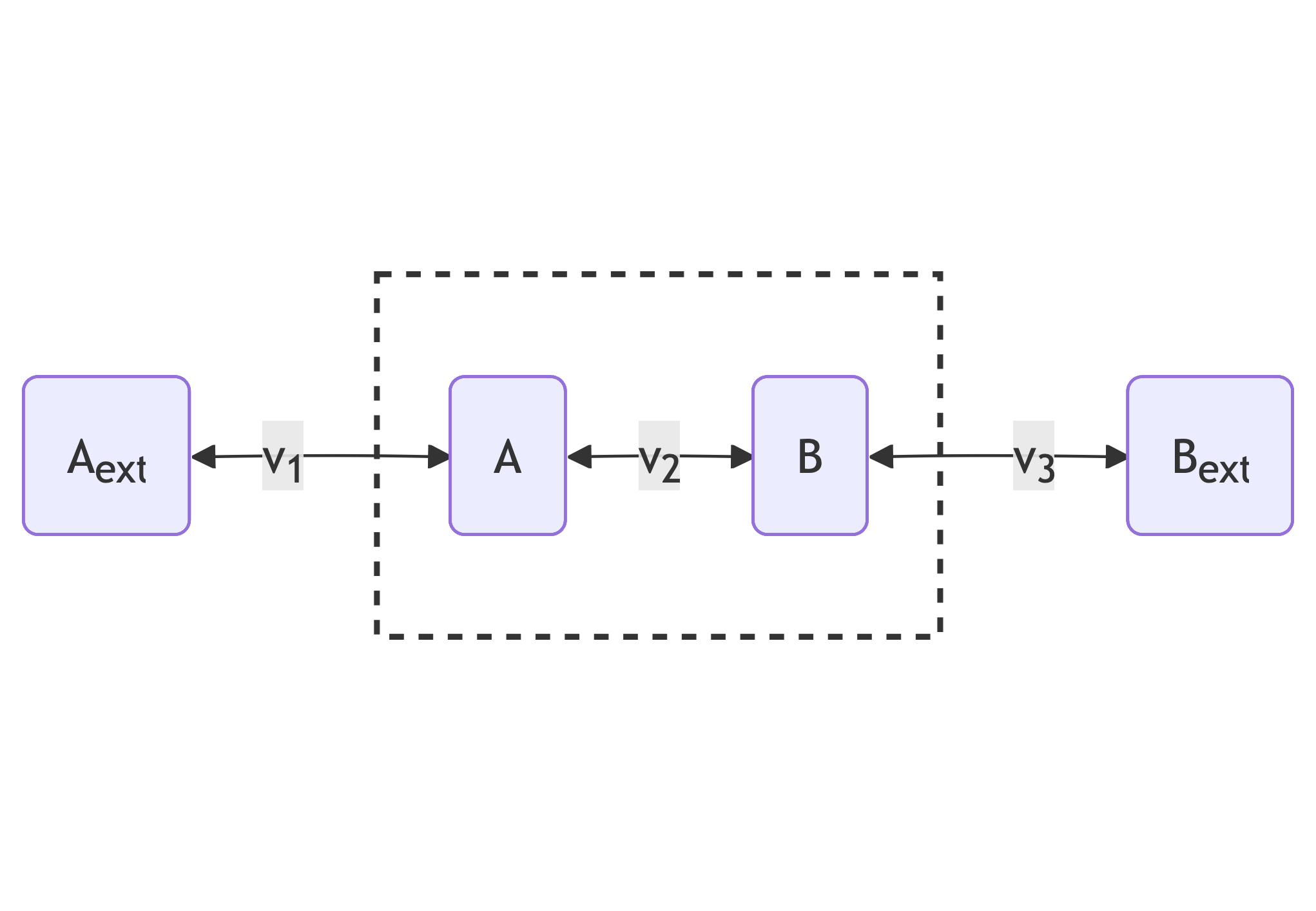
The rates $v_1$, $v_2$ and $v_3$, given internal concentrations
\[x = x_{A}, x_{B}\]and parameters
\[\theta = k^{m}_{A}, k^{m}_{B}, v^{max}, k^{eq}_1, k^{eq}_2,k^{eq}_3, k^{f}_1, k^{f}_3, x^{ext}_A, x^{ext}_{B}\]are calculated as follows:
\[\begin{aligned} v_1(x, \theta) &= k^{f}_1 (x^{ext}_{A} - x_{A} / k^{eq}_1) \\ v_2(x, \theta) &= \frac{\frac{v^{max}}{k^{m}_A} (x_{A} - x_{B} / k^{eq}_2)}{1 + x_{A}/k^{m}_{A} + x_{B}/k^{m}_{B} } \\ v_3(x, \theta) &= k^{f}_3 (x^{ext}_{B} - x_{B} / k^{eq}_3) \end{aligned}\]According to these equations, rates $v_1$ and $v_3$ are described by mass-action rate laws: transport reactions are often modelled in this way. Rate $v_2$ is described by the Michaelis-Menten equation that is a popular choice for modelling the rates of enzyme-catalysed reactions.
The larger network models the mammalian methionine cycle, using equations taken from
For the small linear network, we solved the embedded steady-state problem using the optimistix Newton solver. For the larger model of the methionine cycle we simulated the evolution of internal concentrations as an initial value problem until a steady-state event occurred, using the steady-state event handler and Kvaerno5 ODE solver provided by diffrax. In this case a guess is still needed in order to provide an initial value. Solving a steady-state problem in this way is often more robust than directly solving the system of algebraic equations; see
Code used for these two experiments is in the code repository files benchmarks/methionine.py and benchmarks/linear.py.